Serving LLMs at Scale with vLLM and SGLang
A practical guide to inference architecture, KV cache economics, prefix reuse, routing, and operating vLLM and SGLang under production latency targets.
On this page 22 sections
LLM serving scales by avoiding unnecessary recomputation and managing the state that generation leaves behind. For a conventional Transformer, every output token depends on attention state that grows with the sequence. How an engine allocates, shares, and reclaims that state shapes concurrency, latency, and cost alongside compute and memory bandwidth.
This guide develops that idea from first principles and carries it through production concerns: KV cache sizing, continuous batching, prefix reuse, cache-aware routing, disaggregation, overload control, failure behavior, multi-tenancy, and production design review. The goal is to understand the architectural choices behind vLLM and SGLang and evaluate them against a specific workload.
Version basis: vLLM v0.28.0 and SGLang v0.5.19. Model support, defaults, and feature combinations change quickly; validate them against the exact release and hardware being deployed. The capacity examples below are illustrative calculations, not measured benchmarks.
In this guide
- Requirements and workload
- Inference fundamentals and KV sizing
- Architecture overview, vLLM, and SGLang
- Paging, prefix indexes, and scheduling
- Measuring reuse and benchmarking fairly
- Overload control, routing, and security
- Choosing an engine and production checklist
1. Start with requirements, not engines
Choosing between vLLM and SGLang before characterizing the workload risks producing a benchmark that does not inform the deployment decision. Define the traffic and the service contract first.
1.1 Workload questions
- What is the peak request rate, not merely the daily average?
- What is the distribution of prompt lengths, and what is the p99 rather than the mean?
- What is the distribution of output lengths, and are they bounded?
- What fraction of input tokens matches an earlier request whose KV state is still cached?
- Is the traffic single-turn or multi-turn, and how long do conversations run?
- Is a large system prompt or tool-definition block common to every request?
- Which requests are latency-sensitive and which are batch-like?
- What is the time-to-first-token budget, and the inter-token budget?
- Is the workload interactive (a human waits) or programmatic (a pipeline waits)?
- How many distinct models must be served, and at what relative volume?
- Is the deployment single-tenant or multi-tenant, and is cache isolation required?
- What must happen when accelerator capacity is exhausted: queue, shed, or degrade?
Prompt-length distribution matters more than most teams expect. A workload with a 500-token mean and a 32,000-token p99 behaves nothing like a uniform 500-token workload, because the tail allocates KV cache in proportion to its length and can starve the rest of the batch.
1.2 Example design target
Consider a hypothetical interactive assistant with tool use:
- 400 peak requests per second
- 3,000-token mean prompt, 24,000-token p99 prompt
- 350-token mean output
- A 1,800-token system prompt and tool-definition block on every request
- Multi-turn: mean 6 turns per conversation
- p95 time-to-first-token below 900 ms
- p95 inter-token latency below 45 ms
- 99.95% availability
- Multi-tenant, with cache isolation required between tenants
The naive token arithmetic is:
prefill:  400 req/s × 3,000 tokens =   1,200,000 tokens/second
decode:   400 req/s ×   350 tokens =     140,000 tokens/second
Input-token volume is roughly 8.6 times output-token volume. This makes prefix reuse worth investigating, although token counts alone do not establish the compute cost of either phase.
The shared block changes the picture:
shared prefix:  400 req/s × 1,800 tokens =   720,000 tokens/second
                                             (60% of input token positions)
Up to 60% of input token positions could reuse cached state after warm-up within each replica and tenant cache domain. That is not a 60% reduction in total prefill compute: unmatched suffix tokens still attend to the prefix, and cache misses, block alignment, and isolation reduce realized savings. Section 8 explains how to measure the opportunity.
2. The inference problem both engines solve
2.1 Prefill
Prefill processes prompt tokens, either together or in chunks. Computation across prompt positions parallelizes well, so the phase is often compute-intensive, especially for large token batches. Its output is the first generated token plus the KV cache entries for every prompt position.
Prefill cost grows with prompt length. Dense full attention has quadratic arithmetic cost in sequence length; kernels such as FlashAttention reduce memory traffic without removing that arithmetic. Sliding-window, sparse, and hybrid architectures require a different model.
2.2 Decode
Ordinary autoregressive decode produces one token per sequence per forward pass. With dense models at modest batch sizes, reading weights and KV state often makes it memory-bandwidth-bound. Larger batches amortize weight reads; long contexts increase KV traffic, and MoE models change the weight-access pattern. Speculative decoding can produce multiple accepted tokens per verification step.
This asymmetry is the central fact of LLM serving. Prefill wants large batches of tokens; decode wants large batches of sequences. An engine that serves both from one pool of accelerators must reconcile two opposing appetites.
2.3 Why the KV cache dominates capacity
For a full-attention model, each retained token contributes key and value tensors at every attention layer. A grouped-query-attention model has the following logical KV footprint across all ranks:
bytes per token = 2 × layers × kv_heads × head_dim × bytes_per_elementFor a 70B-class model with 80 layers, 8 KV heads, 128 head dimension, in fp16:
2 × 80 × 8 × 128 × 2 = 327,680 bytes = 320 KiB per tokenA single 8,000-token conversation therefore holds:
8,000 × 320 KiB = 2.441 GiB of KV cacheThat is a key constraint on concurrency. Weights are a fixed cost paid once; KV cache is a per-request cost paid for the entire lifetime of every in-flight sequence.
For an illustrative four-accelerator replica with tensor parallelism of 4, assume 80 GB of usable memory per rank and the following allocation. This example uses decimal GB consistently; production sizing should use the memory and KV capacity reported by the engine:
weights:        140 GB fp16 ÷ 4 ranks        =  35 GB per rank
overhead:       activations, workspace       ≈   5 GB per rank
KV budget:      80 − 35 − 5                  =  40 GB per rank
replica KV:     40 GB × 4                    = 160 GB total
capacity:       160,000,000,000 ÷ 327,680     ≈ 488,281 tokens
concurrency:    488,281 ÷ 8,000 per request  ≈  61 requests
That is about 61 concurrent 8,000-token sequences before block fragmentation and safety headroom. This assumes the eight KV heads shard evenly across four ranks. Other parallel layouts can replicate KV, and MLA, sliding-window, or hybrid models need their own accounting. KV quantization and prefix sharing can increase GPU residency; host-memory tiering expands reusable cache capacity but does not automatically increase active decode capacity.
2.4 Metrics that actually matter
| Metric | Meaning | Bound by |
|---|---|---|
| TTFT | Time to first token | Prefill compute, queue wait, prefix hit rate |
| TPOT / ITL | Average time per output token / gaps between successive tokens | Memory bandwidth, batch composition, scheduling |
| Throughput | Output tokens per second, fleet-wide | Compute, bandwidth, batch size, KV capacity |
| Goodput | Throughput of requests that met their SLO | Everything above, jointly |
TPOT is usually a per-request average after the first token; ITL captures individual token gaps. State the aggregation method when reporting percentiles.
Reporting throughput without the latency distribution it was achieved at is the most common benchmarking error in this domain. A configuration that doubles throughput while pushing p95 inter-token latency past the point of usability has not improved the service.
Goodput is the metric that resists gaming. It counts only the requests that met their contract.
3. Reference architecture
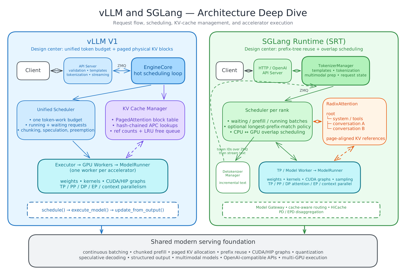
Engine internals at a glance. Features depend on the selected model, backend, and configuration; SGLang’s lpm scheduling policy is optional.
The engine sits inside a broader serving system:
Client
  │
  ▼
API gateway  ── authentication, quota, per-tenant rate limit
  │
  ▼
Router / load balancer  ── cache-aware or round-robin
  │
  ├──────────────┬──────────────┬──────────────┐
  ▼              ▼              ▼              ▼
Engine replica  Engine replica  Engine replica  ...
  │  (vLLM or SGLang)
  │
  ├── scheduler        ── admission, batching, preemption
  ├── KV cache         ── paged physical blocks
  ├── prefix index     ── hash chain (vLLM) or radix tree (SGLang)
  └── model executor   ── TP / PP / EP / DP ranks
  │
  ▼
Tiered cache (optional)  ── host memory, then storage or remote KV
  │
  ▼
Observability  ── per-phase latency, cache hit rate, preemption rate
Two properties of this diagram deserve emphasis before the engine-specific sections.
First, the router is part of the cache architecture, not merely a traffic distributor. Section 12 develops this.
Second, admission control belongs at the engine, not only at the gateway. The gateway can limit request rate; only the engine knows whether KV cache capacity exists to admit a request without preempting an in-flight one.
3.1 Turning a request rate into a replica count
Using the section 1.2 arrival rate and the section 2.3 memory budget, assume fixed 3,000-token prompts, 350-token outputs, and a mean decode interval of 45 ms for this sizing exercise. The p95 SLO is not a substitute for a measured mean. Ignoring queueing and prefill time gives:
mean tokens resident per request  ≈ 3,000 prompt + 175 mean-generated
                                  ≈ 3,175 tokens
mean decode residency            ≈ 350 tokens × 45 ms = 15.75 seconds
concurrent requests (Little's law) ≈ 400 req/s × 15.75 s = 6,300 requests
KV required                      ≈ 6,300 × 3,175 × 320 KiB = 5.96 TiB
replicas of 160 GB KV each        ≈ 40.97, rounded up to 41 replicas
This simplified memory calculation gives 41 four-accelerator replicas, or 164 accelerators, before prefix sharing and operational headroom. It is not a complete fleet recommendation: compute throughput, bandwidth, correlated request lengths, prefill residency, failover, and latency constraints also matter. Reusing 60% of input token positions does not imply a 60% fleet reduction, although sharing the 1,800-token prefix within a replica and tenant domain can materially reduce resident KV.
Treat this arithmetic as a sizing skeleton to be replaced by measurement, not as a prediction. Its purpose is to make the dominant terms visible.
4. vLLM architecture
4.1 Request path
Client → API server → EngineCore → Scheduler → ModelExecutor → workers
                          ▲                                       │
                          └───────── sampled tokens ──────────────┘
vLLM’s V1 engine separates the HTTP/API layer from the engine core, and the engine core coordinates scheduling, model execution, and output processing, with synchronous or asynchronous scheduling paths depending on configuration. Tokenization and detokenization are kept off the critical scheduling path.
4.2 The unified scheduler
vLLM’s defining design decision is to refuse the distinction between prefill and decode as job types. Each request tracks one quantity:
tokens known to the request
− tokens already computed
= tokens that still need model work
Known tokens include prompt tokens, accepted output tokens, placeholders, and speculative draft tokens. Each engine step has a global token budget, and the scheduler allocates that budget across requests until it is exhausted.
With an illustrative budget of 8,192 tokens, the accounting could look like this (the rows do not specify queue order):
| Request | State | Tokens owed | Granted |
|---|---|---|---|
| A | fresh 6,000-token prompt | 6,000 | 6,000 |
| B | mid-generation | 1 | 1 |
| C | mid-generation | 1 | 1 |
| D | fresh 4,000-token prompt | 4,000 | 2,190 |
Request D is processed partially and resumes next step. The unified accounting supports chunked prefill, subject to the configured chunking and admission rules.
The same accounting expresses every case:
| Case | Tokens owed |
|---|---|
| Ordinary decode | 1 |
| Full prefill | prompt length |
| Chunked prefill | whatever the budget allows |
| Prefix cache hit | prompt length − cached length |
| Speculative verification | number of draft tokens |
A prefix cache hit advances the computed boundary without model work. Cache lookup and allocation still require explicit scheduler and cache-manager logic; the remaining model work fits the same token accounting.
The operational consequence is that prompt and decode tokens genuinely compete for one budget. Raising max_num_batched_tokens can improve prefill throughput while increasing inter-token latency for running sequences; measure the tradeoff for the workload. That tradeoff is explicit and tunable rather than buried in phase-transition logic.
When KV space is insufficient, vLLM preempts requests and recomputes them later. A sustained preemption rate is a signal that concurrency or the batched-token limit exceeds what KV memory supports.
4.3 PagedAttention and physical KV allocation
Reserving a contiguous maximum-length KV tensor per request wastes memory because output length is unpredictable. PagedAttention applies operating-system-style indirection:
request's logical block 0 ──> physical KV block 71
request's logical block 1 ──> physical KV block 12
request's logical block 2 ──> physical KV block 98
A block table lets the attention kernel gather non-adjacent physical blocks. The consequences:
- allocation grows with actual sequence length, not maximum length;
- only the final partial block suffers internal fragmentation;
- physical blocks can be shared across requests or candidate continuations;
- freed blocks are recycled without relocating the rest of a sequence.
PagedAttention is both a memory-management scheme and an attention-kernel contract. It is not, by itself, cross-request prefix discovery.
4.4 Automatic prefix caching
vLLM discovers reusable state by hashing each full block of tokens together with its parent block’s hash, plus any additional identity the request carries (LoRA adapter, multimodal inputs, and similar).
block 0 hash = H(tokens[0:16], ∅)
block 1 hash = H(tokens[16:32], block 0 hash)
block 2 hash = H(tokens[32:48], block 1 hash)
Because each hash incorporates its ancestry, two requests sharing a prompt prefix produce identical hashes for exactly the shared blocks and diverge at the first differing block. This represents a prefix tree implicitly, with no parent/child pointers stored anywhere. Lookup is a hash-table probe per block rather than a tree traversal.
Two properties follow from the design. Matching is block-granular: a shared prefix of 20 tokens with a 16-token block size yields one reusable block, not 20 reusable tokens. And eviction operates on cached blocks through an LRU-oriented free-block queue, with reference counts protecting blocks in active use.
4.5 Scaling vLLM
vLLM supports tensor, pipeline, data, and expert parallelism, context parallelism, and KV connectors for external cache transfer. The v0.28.0 release also includes tiered KV offloading, including a disk tier, and encoder/prefill/decode disaggregation work in Model Runner V2.
Treat each topology as a model-, backend-, and connector-specific integration. Compare validated configurations and transfer costs rather than assuming a maturity ranking between engines.
5. SGLang architecture
5.1 Two meanings of the name
The original SGLang paper describes a Python-embedded frontend for structured language-model programs and a runtime that executes them efficiently. The project has since become a general serving framework, and comparisons with vLLM concern SGLang Runtime (SRT), not whether an application uses the frontend DSL.
An application can use the OpenAI-compatible HTTP API, the native /generate endpoint, or the in-process Engine. Taking a dependency on the frontend DSL is a portability decision that should be made deliberately; see section 20.
5.2 Request path
Client → HTTP server → TokenizerManager ──ZMQ──> Scheduler (per rank)
                             ▲                        │
                             │                        ▼
                             │                   Model worker
                             │                        │
                        DetokenizerManager <──ZMQ─────┘
The TokenizerManager owns tokenization, multimodal preprocessing, request state, and result aggregation. Scheduler processes form batches, allocate KV slots, and drive model workers. Detokenization runs in a separate process.
This separation keeps tokenization and incremental detokenization from blocking the GPU scheduling loop, making the hot runtime a pipeline rather than a request/response chain. The cost is more processes, more inter-process message paths, and a correspondingly larger surface for operational failure.
5.3 RadixAttention
SGLang’s cache index is a radix tree — a prefix tree with single-child chains compressed, so each edge holds a sequence of token IDs rather than one token:
root
└── [system prompt, tools]
    ├── [user A, assistant A]
    │   └── [next user turn A]
    └── [user B, assistant B]
        └── [next user turn B]
Nodes point to physical KV locations for their token segments. On arrival, a request finds the longest matching prefix, locks the referenced nodes so they cannot be evicted while in use, computes only the unmatched suffix, and inserts its new aligned KV segments back into the tree. Under memory pressure, evictable leaves are selected by policy, commonly by recency.
The mechanic that earns the name is node splitting. Suppose the tree holds [system, tools, user_A] as one edge and a request arrives as [system, tools, user_B]. The match runs out mid-edge, so the tree splits that edge at the divergence point, promotes [system, tools] to a shared parent, and adds [user_B] as a sibling of [user_A]. Shared structure is discovered incrementally from traffic; nothing is declared in advance.
Eviction targets leaves specifically because an interior node’s KV remains a live prefix for everything beneath it.
“RadixAttention” names the combination of this tree with a paging-aware attention runtime and scheduler. It is broader than an attention kernel.
5.4 Cache-aware scheduling
SGLang exposes cache-aware waiting-queue policies alongside ordinary first-come-first-served scheduling. SRT maintains waiting, prefill, and running/decode state, and its longest-prefix-match (lpm) policy can reorder the waiting queue to group requests that share prefixes.
In v0.5.19, fcfs is the default; lpm is an optional policy, not a requirement of RadixAttention.
Prefill admission considers available token slots, running requests, prompt size, chunk limits, grammar readiness, LoRA compatibility, and cache state jointly.
Reordering is not free. It adds scheduling overhead and it changes fairness: a request whose prefix is unpopular waits longer than it would under first-come-first-served. Mean throughput and TTFT can improve while p99 latency for cache-unlucky requests degrades. Measure the full distribution, with production arrival patterns, before enabling it.
5.5 Overlap scheduling
SGLang’s default scheduler pipelines CPU preparation for the next batch against accelerator execution of the current one, using separate scheduling and forward streams with synchronization barriers to prevent shared-buffer hazards.
This matters when CPU launch overhead would otherwise leave gaps between small decode steps — which is exactly the regime of interactive serving at modest batch sizes. Certain feature combinations require the synchronous path; correctness takes precedence over overlap.
5.6 Chunked prefill and memory admission
Long prompts are split into bounded chunks, reducing peak activation pressure and letting the scheduler interleave prompt work with running decodes. The chunk size is a direct tradeoff:
- larger chunks can improve prefill efficiency while increasing tail inter-token latency;
- smaller chunks improve responsiveness and add scheduler and kernel overhead;
- admitting too many requests still exhausts KV memory during decode.
The relevant controls are --chunked-prefill-size, --max-running-requests, and --mem-fraction-static. The last controls the fraction reserved for model weights and the KV memory pool. Setting it too high leaves insufficient dynamic memory for activations and workspace, risking OOM errors; setting it too low reduces available KV capacity. Tune it against measured headroom.
5.7 Hierarchical cache (HiCache)
L1: GPU KV        lowest latency, smallest capacity
  ▲
  ▼
L2: host memory   larger, PCIe or NVLink transfer cost
  ▲
  ▼
L3: storage / remote KV   largest, highest latency
HiCache extends the radix-managed cache into host-memory and optional storage tiers. Storage backends and transfer paths are separate integration choices; validate the backend supported by the pinned release and deployment.
The governing question is not whether a hit occurs but whether a hit is cheaper than recomputation. Fetching the example’s 2.441 GiB of KV at an effective 20 GB/s takes about 131 ms before other overhead; recomputing an 8,000-token prefill may cost less. HiCache pays off for long-context and multi-turn workloads whose working set exceeds GPU KV, and it can lose to recomputation for short prefixes on fast accelerators.
It is not free capacity. Host memory must be budgeted per rank, interconnect or storage bandwidth can become the bottleneck, and aggressive write-through or prefetch policies interfere with model traffic.
5.8 Scaling and disaggregation
Beyond TP, PP, DP, and EP, SGLang offers several specialized layouts:
- DP attention: attention processes different batches per replica while FFN/MoE computation stays tensor- or expert-parallel. For MLA/MoE models this avoids the KV duplication that tensor parallelism would otherwise impose, making it worth evaluating independently of prefix reuse. Support and benefits depend on the model and parallel layout.
- Expert parallelism with selectable all-to-all backends and expert load balancing.
- Attention context parallelism for long sequences.
- PD disaggregation: dedicated prefill and decode workers exchanging KV state over Mooncake or NIXL behind a router.
- EPD disaggregation: multimodal encoders scaled independently of prefill and decode.
PD disaggregation directly addresses the section 2.2 asymmetry: prefill is often compute-heavy while decode is often bandwidth-heavy. Separating them allows independent capacity tuning and can protect decode from prefill interruptions. It introduces routing, KV-transfer bandwidth, additional failure modes, and materially harder capacity planning. Treat published PD guidance as topology-specific rather than as a default recipe.
5.9 Model gateway
SGLang’s gateway provides cache-aware routing and load-balancing policies around engine workers, with topology-specific integrations for distributed serving. Evaluate worker discovery, health checks, retries, admission limits, and observability as part of the gateway configuration; capabilities and API coverage depend on the gateway version.
Its significance is architectural rather than convenient, and section 12 explains why.
6. PagedAttention versus RadixAttention
The frequent framing — paging versus radix — is a category error. Both engines page physical KV; both index reusable prefixes. They differ in how reuse is found and scheduled.
| Question | vLLM | SGLang |
|---|---|---|
| How is KV stored physically? | Paged blocks with a block table | Paged blocks with a pool |
| How is reusable state found? | Chained block hashes plus identity | Walk a compressed radix tree keyed by token sequences plus identity |
| Lookup cost | Hash probe per block | Tree walk proportional to matched length |
| Is the prefix structure explicit? | No — implied by hash ancestry | Yes — nodes, edges, parents, children |
| Match granularity | Full blocks | Page-aligned radix segments |
| How is active sharing protected? | Reference counts on physical blocks | Locks and reference state on nodes and pool entries |
| What is evicted? | Cached blocks via LRU-oriented free queue | Evictable leaves and subtrees by policy |
| Waiting-queue policy | FCFS or priority; prefix hits reduce scheduled work | FCFS by default; optional cache-aware policies such as lpm |
| Can cache exceed GPU memory? | KV connectors and tiered offloading | HiCache host-memory and storage tiers |
The explicit tree naturally represents shared branches and supports SGLang’s locality-oriented scheduling and cache policies. Chained hashes provide an expected constant-time hash-table probe per block, with total lookup work growing with prefix length. Cache-aware scheduling and tiering are not exclusive to either data structure; compare the implemented policies and their measured behavior.
So the engineering question is not “paging or radix” but:
- Does the traffic contain enough reusable prefix to make cache policy a major factor?
- How much reuse survives the chosen routing policy across replicas?
- Does the working set exceed GPU KV, making tiering worthwhile?
- Are the specialized MoE or disaggregation layouts needed independently?
7. Continuous batching and chunked prefill
Static batching — wait for N requests, run them to completion together — wastes capacity because sequences finish at different times, leaving idle slots until the longest completes.
Continuous batching admits new work as slots free:
step k    : [A decode] [B decode] [C decode] [D prefill chunk]
step k+1  : [A decode] [B decode] [C done  ] [D prefill chunk]
step k+2  : [A decode] [B decode] [E prefill] [D decode]
Both engines implement it; it is table stakes rather than a differentiator.
Chunked prefill is what makes continuous batching tolerable for interactive traffic. Without it, a single 32,000-token prompt monopolizes a step and stalls every in-flight decode, producing a visible inter-token latency spike for unrelated users. With it, that prompt is spread across steps and the stall is bounded by the chunk size.
The tuning rule follows directly: tune chunk size against the inter-token-latency budget while measuring its throughput cost. Set it from the ITL budget, then verify throughput is acceptable, rather than the reverse.
8. Prefix reuse: measure before choosing
The most common analytical error is reasoning from prompt appearance rather than measured token overlap. Both engines cache prefixes, so the mere existence of a system prompt does not favor either.
Compute one number from a real traffic sample: the token-weighted fraction of input tokens that match a reusable prefix from an earlier request. Replay requests in arrival order and estimate cache residency from available memory, the working set, and eviction behavior. Include cache warm-up and the routing policy.
for each request r in arrival order:
    shared[r] = longest block/page-aligned prefix whose KV was computed
                by an earlier request and remains eligible in this cache domain
reuse_fraction = Σ shared[r] / Σ input_tokens[r]
An overlap-only replay is an upper-bound estimate, not an observed engine hit rate. Cache identity must include the model revision, adapter and multimodal context, and tenant boundary where required. Validate the estimate against token-level hit metrics under load.
| Observed pattern | Evaluation focus |
|---|---|
| Little reusable prefix | Model support, kernels, batching, and operating cost |
| Substantial reuse on one replica | Benchmark both cache policies; measure TTFT and fairness at p99 |
| Substantial reuse across many replicas | Include routing, warm-up, replication, and eviction in the benchmark |
| Working set exceeds GPU cache | Compare tiered-cache transfer cost with recomputation |
Three qualifications matter. Arrival spacing and eviction both affect reuse: lower load lengthens gaps between requests but may also reduce cache pressure, so off-peak behavior must be measured rather than assumed. Replaying identical prompts back-to-back can overstate production reuse. Multi-turn conversations produce reuse that is high but serialized, since turn N reuses turn N−1’s state only if that state survives the user’s think time. And per-tenant isolation partitions the cache, so a multi-tenant deployment’s effective reuse is computed within tenants, not across them.
9. Capacity planning
Work forward from the section 2.3 model.
Step 1 — establish bytes per token. Compute it from the model’s actual layer count, KV head count, and head dimension. Do not estimate it; a factor-of-two error here invalidates the entire plan. FP8 KV storage roughly halves the raw tensor bytes relative to FP16/BF16 where supported; account for metadata and validate accuracy, kernels, and model compatibility.
Step 2 — establish per-replica KV budget. Subtract sharded weights, activation/workspace requirements, graph allocations, and safety headroom from usable accelerator memory. Prefer the engine’s reported KV token capacity and avoid double-counting a static reservation that already includes its KV pool.
Step 3 — derive token capacity and concurrency. KV budget divided by bytes per token gives resident token capacity; divide by mean resident tokens per request for concurrency.
Step 4 — apply Little’s law. Concurrency equals arrival rate times mean residency time, and residency is dominated by output length times inter-token latency. This is where output-length distribution enters capacity planning, and why unbounded max_tokens is a capacity risk rather than a generosity.
Step 5 — add headroom for the tail. A p99 prompt of 24,000 tokens consumes eight times the KV of a 3,000-token mean prompt. Plan for the length distribution, not its mean.
Step 6 — subtract expected prefix savings, conservatively. Shared prefixes reduce both prefill compute and resident tokens, when compatible requests use the same cache domain. Tiered reuse can reduce recomputation without increasing simultaneous GPU residency. Discount the section 8 measurement by expected routing efficiency before spending it.
Two derived quantities are worth monitoring as capacity signals in their own right: the preemption rate, which indicates admission exceeding KV capacity, and the cache hit rate, which indicates whether the reuse assumed in planning is materializing.
10. Benchmarking fairly
10.1 State the decision and SLO first
A benchmark that does not name the decision it informs will not inform it. Write down the SLO — for example, “p95 TTFT under 900 ms and p95 ITL under 45 ms” — before generating load, and report throughput at that SLO.
10.2 Hold these constant
- model weights, revision, and quantization scheme
- accelerator model, count, and interconnect topology
- tensor/pipeline/expert parallel degrees
- maximum sequence length and maximum batched tokens
- sampling parameters, including temperature and
max_tokens - tokenizer and chat template
- client implementation and concurrency model
- warm-up procedure and cache state at measurement start
Cache state is the one most often neglected. A cold-cache run and a warm-cache run of the same configuration can differ by more than the two engines differ from each other.
10.3 Use a workload matrix
| Axis | Values worth testing |
|---|---|
| Prompt length | short, mean, p99 |
| Output length | short, mean, long |
| Prefix sharing | none, partial, heavy |
| Arrival pattern | steady, bursty, diurnal |
| Concurrency | below, at, above capacity |
| Multi-turn | single-turn, 6-turn conversation |
The prefix-sharing axis is what makes an LLM serving benchmark different from a generic throughput benchmark, and omitting it is how teams conclude the engines are equivalent.
10.4 Report a frontier, not a number
Sweep concurrency and plot throughput against p95 latency. The result is a curve, and the engines may trade places along it. A single operating point conceals which one degrades more gracefully past the knee — which is the property that matters during an incident.
10.5 Common mistakes
- replaying identical prompts, which measures cache hit paths rather than the workload
- measuring with unbounded
max_tokens, letting output length drift between runs - comparing a tuned configuration of one engine against defaults of the other
- benchmarking from a single client process that becomes the bottleneck
- reporting mean latency for a workload whose tail is the actual constraint
- running to a fixed request count rather than a fixed duration, so faster configurations see less cache warming
11. Overload control and tail latency
Accelerator capacity is inelastic on the timescale of a traffic spike. When demand exceeds it, the system chooses among queueing, shedding, and degrading — and if it does not choose deliberately, it queues until timeouts cascade.
Bound the queue explicitly. An unbounded admission queue converts an overload into a latency collapse in which every request eventually times out after consuming capacity. A bounded queue with fast rejection preserves goodput for admitted work.
Reject rather than preempt, past a threshold. Preemption discards completed prefill work that must be recomputed, so a system that preempts under sustained overload does strictly more total work than one that admits fewer requests.
Cap output length per request. Unbounded generation makes residency unbounded, and residency drives concurrency. This is the cheapest available protection.
Separate interactive and batch traffic. They have incompatible appetites (section 2.2) and incompatible SLOs. Serving them from one replica pool means batch prefills injecting ITL spikes into interactive sessions. Separate pools, or PD disaggregation, address this structurally.
Degrade deliberately. Define application-compatible output caps, bounded queueing, load shedding, and—where the product contract allows it—routing to a smaller model. Benchmark each fallback. Changes to speculation or chunk size are engine- and version-dependent and may require a rolling restart; do not assume they are safe runtime switches or that they reduce load in every workload.
12. Multi-replica cache locality
This section is the one most likely to change a deployment decision, and it concerns the router rather than the engine.
Routing changes cache warm-up, replication, and session locality. A universal system prefix behaves differently from conversation-specific history:
8 replicas, round-robin, one shared 1,800-token system prefix:
  the prefix is computed and stored once per replica/cache domain
  after warm-up, each replica can retain a high hit rate for that prefix

Session history cached on one of 8 replicas, with uncorrelated routing:
  a later turn has roughly a 1/8 chance of reaching that replica
  unless history is already present elsewhere or transferred
Round-robin does not divide steady-state reuse of a universal prefix by eight. It replicates that prefix’s memory cost and warm-up work. Under short cache residency, frequent restarts, or many tenant-specific prefixes, those costs become more significant.
A later conversation turn sent elsewhere may still hit the shared system prefix, while recomputing the conversation-specific suffix. Session affinity preserves that additional reuse. Three consequences follow.
Session affinity is a useful baseline for multi-turn traffic. Route a conversation to the replica holding its history. This is achievable with any conventional load balancer using a consistent hash on session identity, and it captures most of the multi-turn benefit without any engine-specific machinery.
Cache-aware routing is the stronger form. Route by content prefix rather than session identity, so unrelated users sharing a system prompt also land together. SGLang provides gateway policies for this. vLLM can also participate in cache-aware deployments through external routers and KV-cache event integrations; evaluate the complete routing stack.
Affinity trades against balance. Perfect locality sends all traffic for a popular prefix to one replica and overloads it. One useful approach is power-of-two-choices routing among replicas holding a prefix: pick the less loaded of two cache-holding candidates. Any affinity scheme needs a load-based escape valve, or a viral prefix becomes a hotspot.
The practical summary: if the deployment has several replicas and prefix-heavy traffic, the routing layer can matter as much as the engine-level cache index. Single-replica results should be validated again with the intended routing policy and fleet size.
13. Multi-region considerations
KV cache does not travel well. It is large (section 2.3), and it is tied to a specific model revision, parallelism layout, cache format, runtime/backend compatibility, and transfer implementation. Cross-region KV replication is rarely worthwhile.
Consequently:
- Treat each region as an independent cache domain with its own warm-up cost.
- Route conversations to a home region and keep them there; a cross-region failover may require re-prefilling active sessions, which is a capacity event, not merely a latency event.
- Size regions for their own peak, not for a global average, because a region absorbing failover traffic must also absorb the re-prefill burst.
- Replicate the model artifacts and configuration, which are static, rather than the cache.
14. Failure modes and degradation
| Failure | Effect | Mitigation |
|---|---|---|
| KV exhaustion | Preemption, then latency collapse | Bounded admission, output caps, preemption alarm |
| Cache loss on replica restart | Re-prefill burst, TTFT spike | Staggered restarts, gradual traffic ramp |
| Router loses cache awareness | Session and less-common prefix reuse can fall | Monitor hit rate by traffic class alongside latency |
| One long prompt in a batch | ITL spike for unrelated users | Chunked prefill, prompt length cap |
| Hot prefix | One replica saturates | Power-of-two routing among cache holders |
| HiCache tier slower than recompute | Latency worse with cache | Measure hit cost against recompute cost; disable tier |
| Model artifact mismatch across replicas | Inconsistent outputs, silent | Pin revisions, assert on load, contract tests |
| Speculative decoding acceptance collapse | Throughput drops below baseline | Monitor acceptance and goodput; use a validated rollback path |
| PD KV transfer saturation | Decode starves despite idle prefill | Monitor transfer bandwidth separately |
Two of these deserve emphasis because they are silent. A cache hit that is slower than recomputation degrades the service while every cache metric looks healthy. And speculative decoding with a collapsed acceptance rate consumes draft compute for no benefit — monitor acceptance rate together with end-to-end goodput and draft overhead.
Restart behavior is the failure mode most often discovered in production. A replica that restarts with an empty cache and immediately receives its full share of traffic can trigger a prefill burst, saturate compute, and increase memory pressure and preemption — turning a routine restart into an incident. Ramp traffic to a cold replica.
15. Observability
Instrument these, and alarm on the ones marked as leading indicators:
| Signal | Why | Leading? |
|---|---|---|
| TTFT distribution, p50/p95/p99 | The contract for interactive use | |
| ITL distribution | The other half of the contract | |
| Prefix cache hit rate | Validates the capacity plan | Yes |
| Preemption rate | Admission exceeding KV capacity | Yes |
| KV utilization | Headroom before preemption | Yes |
| Queue depth and wait time | Distinguishes queueing from compute | Yes |
| Running batch size | Explains ITL movement | |
| Tokens/second, prefill and decode separately | Aggregates hide the asymmetry | |
| Speculative acceptance rate | Detects silent regression | Yes |
| Per-tenant token consumption | Attribution and quota | |
| HiCache tier hit rate and transfer latency | Whether tiering is earning its cost |
Separating prefill from decode throughput is the highest-value change most teams can make to an existing dashboard. A single aggregate tokens-per-second number moves for reasons that cannot be diagnosed, because it mixes phases with different compute and bandwidth behavior.
Track token-weighted cache hit rate against a traffic-aware baseline. It can reveal a routing regression, a restart storm, or a traffic-shape change before latency degrades enough to breach the SLO.
16. Security and multi-tenancy
Prefix cache sharing is a cross-tenant channel. If two tenants’ requests can share cached prefixes, timing differences reveal whether another tenant has submitted a given prompt prefix. Where isolation is required, partition the cache by tenant and accept the reduced hit rate — and account for that reduction in the section 8 measurement rather than discovering it in production.
Structured output and tool parsing are application contracts. If the application depends on a specific tool-call format or reasoning-output shape, that dependency must be covered by contract tests that run against the engine version being deployed. Both engines have changed these formats across releases.
Determinism is not free. Outputs can vary with batch composition, because floating-point reduction order changes. If bit-identical outputs across batch sizes are required, that is a constraint to validate explicitly on either engine rather than an assumption.
The engine is not an authorization boundary. Quota, rate limiting, and tenant identity belong at the gateway. The engine’s admission control protects capacity, not access.
17. Production design review: ten questions
17.1 What is the latency budget, split by phase?
Name a TTFT budget and an ITL budget separately, because they are bound by different resources and tuned by opposing controls. A single end-to-end budget cannot be allocated to an engine configuration.
17.2 What is the measured prefix reuse fraction?
Token-weighted, from real traffic, within a window matching cache residency, computed within tenant boundaries if isolation is required. Use the ordered replay and observed hit metrics in section 8; a large system prompt alone does not establish realized reuse.
17.3 What is the KV cache size per token, and per replica?
Computed from the model’s real layer and KV-head counts, not estimated. Use it to establish the memory constraint on concurrency, then validate compute, bandwidth, and latency limits.
17.4 What happens when KV memory is exhausted?
Specify a bounded queue, fast rejection, output caps, and preemption monitoring. Sustained recomputation under overload consumes capacity that could serve admitted work.
17.5 Does the router preserve cache locality?
Evaluate session affinity for conversation history and content-aware routing for shared prefixes. Compare fleet-wide cache hits, balance, and warm-up under the actual routing policy. Section 12 distinguishes universal-prefix reuse from session locality.
17.6 What happens when a replica restarts cold?
Traffic must ramp. A cold replica receiving full traffic can trigger a prefill surge and increased preemption. Staggered restarts and a ramp are the mitigation.
17.7 How is a hot prefix prevented from saturating one replica?
Power-of-two choices among replicas holding the prefix, with a load-based escape valve. Pure affinity converts a popular prefix into a hotspot.
17.8 Are interactive and batch traffic isolated?
Separate pools or disaggregation provide strong isolation. If pools are shared, validate chunking, priority policies, and admission limits against interactive tail-latency SLOs under batch load.
17.9 What is the maximum output length, and is it enforced?
Unbounded output means unbounded residency, which means concurrency cannot be planned. An enforced cap is the cheapest capacity protection available.
17.10 Can the system degrade without becoming unavailable?
Document the output limits, admission policy, routing fallbacks, and load-shedding behavior. Identify which controls are safe at runtime and which require a tested rolling configuration change.
18. Choosing between them
18.1 Start with vLLM when
- a strong general-purpose baseline with broad integrations is wanted;
- the required model is supported by vLLM’s native implementation or Transformers modeling backend;
- offline Python inference matters as much as HTTP serving;
- the surrounding stack already standardizes on vLLM;
- one serving ecosystem is needed for generation and supported pooling or multimodal tasks, with endpoint and model compatibility validated;
- measured prefix reuse is low and the decision turns on kernels, batching, and model support.
18.2 Put SGLang early in the evaluation when
- large prompt prefixes repeat across requests or conversation turns, and locality can be preserved by routing;
- the useful prefix working set exceeds GPU KV capacity and HiCache is viable;
- a tuned MoE service using DP attention, EP, and specialized all-to-all paths is the target;
- PD or EPD disaggregation is part of the intended topology;
- SGLang’s cookbook has a validated recipe for the exact model and hardware.
Note that two of these — MoE layouts and disaggregation — have nothing to do with prefix reuse. Their value can be independent of shared prefixes, so evaluate them separately from cache reuse. vLLM also supports specialized parallel and disaggregated layouts; compare recipes for the exact model and hardware.
18.3 Require a proof-of-concept for either engine when
- a required model/quantization/LoRA/speculation combination is only partially supported;
- multi-node networking is slower or less reliable than the reference topology;
- the service is multi-tenant and cache isolation is required;
- tool parsing or reasoning-output format is an application contract;
- determinism across batch sizes is required;
- accelerator support arrives through a community plugin or a recently added backend.
18.4 The usual outcome
The common sensible result is not a permanent organization-wide winner. Teams standardize an OpenAI-compatible gateway, keep contract tests and observability engine-agnostic, and select an engine per model and workload.
A stable gateway contract reduces migration effort. OpenAI-compatible APIs still differ in supported parameters, streaming details, tool parsing, and model behavior. Keep contract tests across engines; adopt native endpoints or frontend features when their benefit justifies the additional integration work.
19. Practical implementation sequence
- Characterize traffic: prompt and output length distributions, turn counts, arrival pattern.
- Measure the prefix reuse fraction (section 8) before evaluating any engine.
- Compute KV bytes per token and per-replica capacity (section 2.3).
- Size a fleet skeleton with Little’s law (section 3.1).
- Stand up both engines with matched configuration; verify output correctness against contract tests before measuring performance.
- Benchmark the workload matrix (section 10.3) and plot frontiers, not points.
- Decide the routing strategy — it may matter more than the engine choice.
- Instrument the section 15 signals, especially cache hit rate and preemption rate.
- Load-test past capacity to observe degradation, not only up to capacity.
- Test cold-start ramp and replica restart behavior explicitly.
- Only then tune: chunk size from the ITL budget, batched tokens from the TTFT budget.
- Re-verify feature-level assumptions on every engine upgrade.
20. Design principles to retain
KV cache is a core capacity constraint. Bytes per token and available memory bound residency; compute, bandwidth, and latency determine how much of that capacity can be used productively.
Prefill and decode are different workloads. Prefill is often compute-heavy and decode often bandwidth-heavy. Measure both phases because their bottlenecks shift with model, context, and batch size.
Both engines cache prefixes. Compare their scheduling policies, cache implementations, tiering integrations, and routing behavior under the intended workload.
The router is part of the cache. Validate single-replica reuse across the fleet, including warm-up, replication cost, session locality, and load balance.
Measure reuse; do not assume it. Token-weighted, from real traffic, within tenant boundaries.
Bound everything that residency depends on. Output length, queue depth, admitted concurrency. Unbounded residency makes capacity unplannable.
A cache hit is only a win if it beats recomputation. This is not automatic for tiered caches.
Keep the gateway boundary clean. It is what makes the engine decision reversible.
Report goodput at an SLO. Throughput without a latency distribution is not a result.
21. Compact review checklist
- TTFT and ITL budgets stated separately
- Prompt and output length distributions measured, including p99
- Prefix reuse fraction measured token-weighted from real traffic
- KV bytes per token computed from actual model dimensions
- Per-replica KV budget and token capacity derived
- Fleet sized with Little’s law, with tail headroom
- Output length capped and enforced
- Admission queue bounded, with fast rejection
- Preemption rate alarmed as a capacity signal
- Cache hit rate alarmed as a leading indicator
- Prefill and decode throughput reported separately
- Routing policy validated for session locality and shared-prefix reuse
- Hot-prefix protection via load-aware affinity
- Interactive SLOs protected under batch load
- Cold-replica traffic ramp implemented and tested
- Degradation controls and rolling-change requirements documented
- Cache isolation verified if multi-tenant
- Tool-call and structured-output formats covered by contract tests
- Determinism requirements validated if applicable
- Benchmarks report frontiers at a stated SLO
- Feature-level assumptions re-verified against pinned engine versions
Sources and further reading
- vLLM v0.28.0 release notes: version-specific changes, including tiered offloading and disaggregation.
- vLLM V1 scheduler source, v0.28.0: scheduling budgets, cache lookup, admission, and preemption.
- vLLM automatic prefix caching design: block hashing, cache identity, and isolation.
- Efficient Memory Management for Large Language Model Serving with PagedAttention: the original vLLM/PagedAttention paper.
- SGLang v0.5.19 release notes: current release scope and model-specific recipes.
- SGLang server configuration, v0.5.19: memory allocation, scheduling policies, and feature controls.
- SGLang: Efficient Execution of Structured Language Model Programs: RadixAttention and the original frontend/runtime architecture.
For a closer look at attention state itself, see how the KV cache makes LLM inference possible.